← 返回列表
🔗 原文
无需微积分的PID(几乎)——在电子表格中实现
Calculus-Free PID (Almost) in a Spreadsheet

PID controllers are everywhere. They regulate temperature, motor speed, power supplies, positioning systems, process equipment, and probably a dozen things within arm’s reach of you right now.

They’re also frequently explained with enough calculus to make them seem more mysterious than they really are. Granted, the I and D in PID stand for calculus terms, but they are easy enough to build into a spreadsheet. Grab a copy and keep it open while you read this post.

The Google Sheet implements a simple simulated PID controller along with a simulated process — the thing we’re trying to control. You can change the controller gains, alter the process, introduce disturbances, and watch what happens without compiling anything or wiring up a heater that might accidentally become a toaster.

The three letters in PID stand for Proportional, Integral, and Derivative. If your calculus is rusty, integral is just how much is building up over time, and the derivative is how much changed just now. Each operates on the error:

error = setpoint - process value

The setpoint is where we’d like the system to be, the process value (PV) is where it actually is, and we would obviously like the error to be zero. Proportional is the most obvious method of control. The more we are off, the more we adjust. The closer we are to the setpoint, the less proportional output we need.

Integral, on the other hand, looks at a running tally of errors. Finally, derivative measures how much things have changed from the last time we looked. The basic cycle time for the spreadsheet is set by dt, which, by default, is 0.1 seconds. Therefore, it takes ten spreadsheet rows to cover an entire second.

Suppose we’re controlling temperature and want it to be 20 degrees. If the temperature is 15, the error is +5. If it’s 22, the error is -2. Our controller’s job is to turn that error into an output. That output affects something — a heater or a motor speed or whatever — that can change the process value. So for a temperature example, the output might drive a heating resistor, and the process value is measured by a thermistor.

The PID tries to drive the heater so that the process value is as close as possible to the setpoint. To the PID algorithm, the actual units of the output and the process values are immaterial. The spreadsheet limits output from 0 to 100 and, presumably, that would be a percentage of voltage or a PWM duty cycle. The setpoint and process value might be in degrees C or F. But the algorithm doesn’t really care.

First, Just P

Make sure the Model drop-down is set to DEFAULT. We’ll begin by setting:

Kp = 4
Ki = 0
Kd = 0

Set the initial process value to 0, the setpoint to 20, the process gain to 1, and the time constant to 2 seconds. With only the proportional term operating, the controller is particularly easy to understand:

output = Kp × error

At the beginning, the error is 20, so the controller asks for an output of 80 (that is, 4 times 20). However, the process doesn’t instantly jump to 80. Our simulated plant is a first-order system implemented essentially as:

PVnew = PVold + dt/tau × (Kprocess × output - PVold)

The actual spreadsheet has extra terms for a bias and disturbance, but you’ll usually leave those at zero. That’s a useful generic model for a surprising number of real things. Turn up a heater, and the temperature approaches a new value gradually. Apply voltage to a motor and its speed doesn’t change instantaneously. Charge a capacitor through a resistor, and you’ve seen exactly this sort of exponential behavior before.

As the process value rises, the error gets smaller. Because the error gets smaller, the proportional controller reduces its output. This works. At least, mostly.
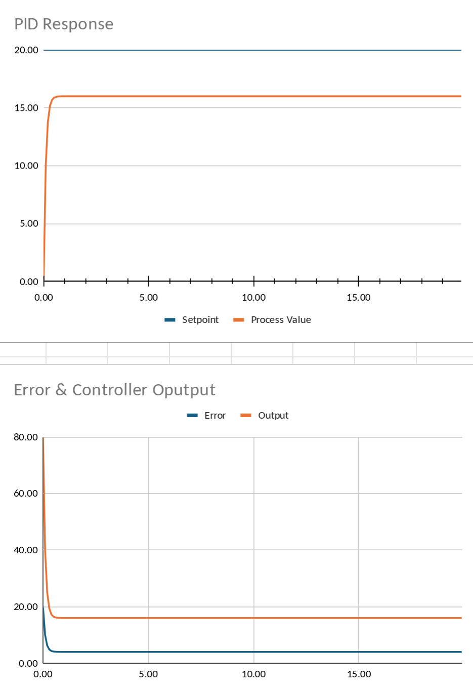
Proportional can’t quite get there.

Watch where it eventually settles. With the suggested values, the process value winds up around 16 even though our setpoint is 20. Why? At a process value of 20, the error would be zero. A proportional controller presented with zero error produces zero output. But this particular process needs an output of 20 to remain at 20. Therefore, it can’t ever quite get there.

This is the classic steady-state error of proportional-only control. We could crank Kp upward. Try Kp=8. The process gets much closer to the setpoint. But continually increasing proportional gain isn’t a universal solution. Eventually real systems start overshooting, oscillating, amplifying noise, or otherwise expressing their displeasure. We need another term.

Remember the Error

Set Kp back to 4 and try:

Ki = 0.5

The integral term looks at not just the error right now, but the error accumulated over time. In the spreadsheet there’s an Integral State column. Each row does approximately this:

integral = previous_integral + error × dt

and the I contribution becomes:

I = Ki × integral

Now consider our P controller sitting stubbornly below the desired value. As long as some positive error remains, the integral keeps growing.

That gradually increases the controller output until the remaining error disappears. Instead of settling around 16, the process now creeps all the way toward 20. This demonstrates one of the major reasons integral control exists: it eliminates persistent offset. It also gives us a good excuse to disturb the system.
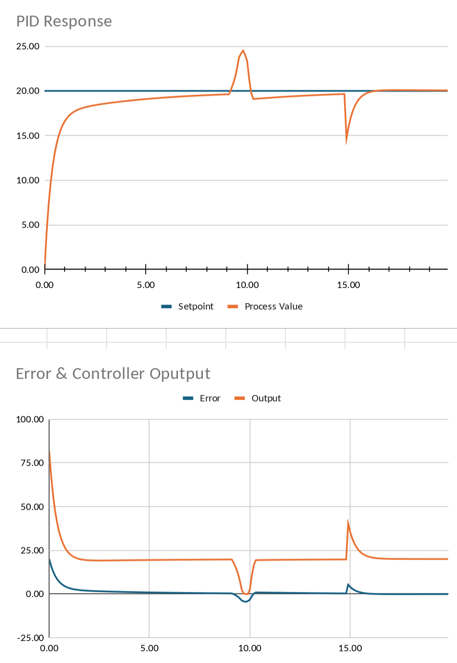
Select the user process model and set User Model # to 1. This will let you disturb the process value by entering numbers into the User1 column. Leave the first bit of the User1 column at 0. But somewhere farther down the simulation, put a disturbance into that column — perhaps -5. If you are feeling especially salty, try a sequence like: 0.5, 0.75, 1, 1.5, 2, 1.5, 0.75, 0.5, -1, -1, -0.5. That sequence should already be in the template’s User1 column.
You can imagine that as opening a refrigerator door, suddenly putting a mechanical load on a motor, or connecting another load to a regulated power supply.

A proportional-only controller reacts immediately, but once things settle, it again tolerates a permanent error.

The integral controller doesn’t. If the process remains below the setpoint, integral action continues increasing until the disturbance has been compensated. That’s a powerful trick. Unfortunately, integral control has tricks of its own.

Too Much of a Good Thing

Integral action remembers errors, but memories aren’t always helpful. The derivative term responds to how rapidly the error is changing:

D = Kd × (error - previous_error) / dt

If proportional control asks, “How far away are we?”, derivative control asks, “How fast are we approaching?” Or, more precisely in this case, “How fast is the error changing?”

Make the simulated process faster by changing its time constant from 2 to about 0.8 seconds. Then try something deliberately more aggressive:

Kp = 8
Ki = 1
Kd = 0
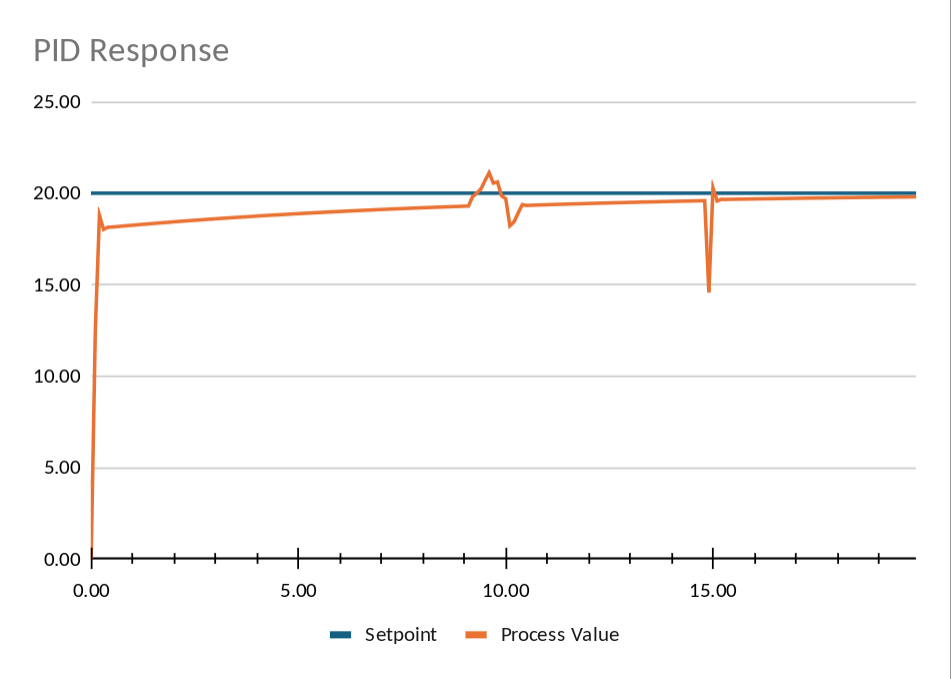
Overshoot in user model #1

The response now gets to the setpoint quickly, but it overshoots it. The problem is easy to see in the spreadsheet. While the process is racing upward, it remains below the setpoint, so the integral continues accumulating positive error. By the time we arrive at the destination, the integral term is still pushing. Depending on the process and gains, the result may be a little overshoot, a lot of overshoot, or sustained oscillation.

Since the default plant is only first-order, derivative action doesn’t have much to work with. User Model 2 adds another lag, using the USER2 column as an intermediate process state. That produces more phase lag and makes aggressive PI tuning more prone to overshoot.
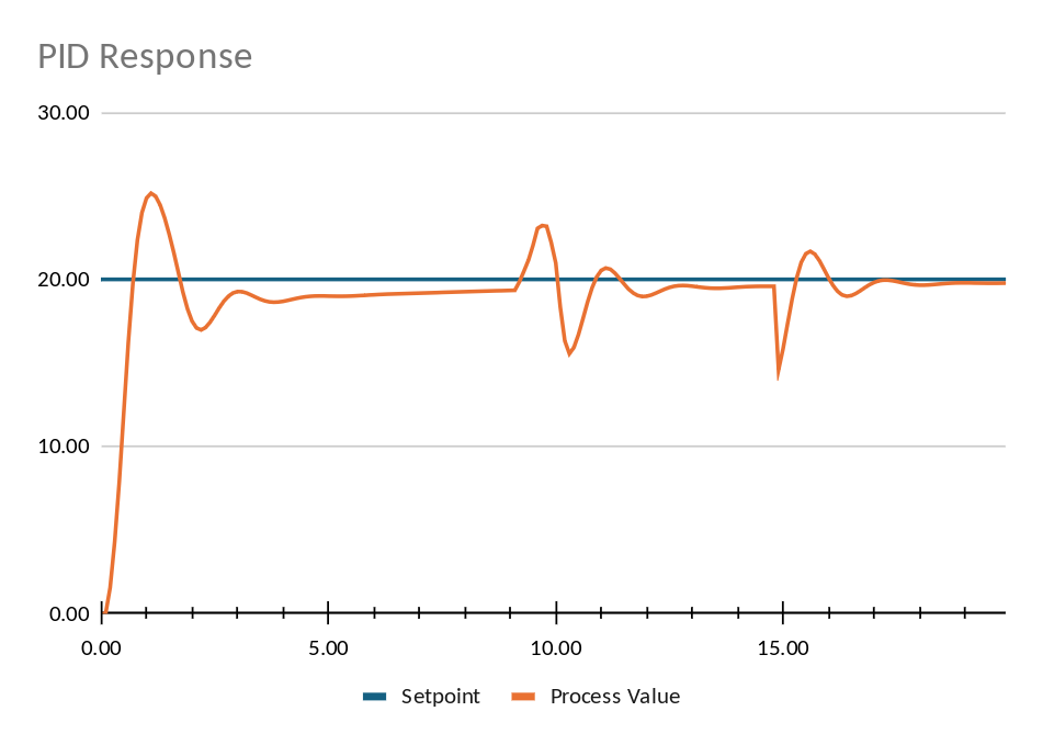
Overshoot observed in model 2.

Switch to User Model 2 and start with Kd=0. Then note the peak process value. Then try Kd=0.2, 0.5, and perhaps 1.0. Try some negative values. You will find that there is a range where the peak overshoot is reduced slightly, but keep going and the response starts to ring. Push Kd far enough, and the derivative term becomes part of the problem rather than part of the cure. The graphs autoscale, so sometimes what looks like a peak the same size (or even bigger) is really smaller than the previous result. Be sure to read the numbers.

That’s the basic PID balancing act. P reacts to the error that exists now. I reacts to error that has existed for a while. D reacts to where the error appears to be heading. Put all three together, and you have a controller that may respond strongly, eliminate steady-state error, and anticipate rapid changes. However, sometimes you are better off with, for example, just PI or even just pure proportional control. Having the algorithm in a spreadsheet form is a nice way to experiment, especially if you can model the system’s behavior.

It’s Only a Spreadsheet

You can add your own models by modifying USR_PROCESS to call your function or just modify one of the existing ones. DEF_PROCESS is just a simple lag model. USR_PROCESS0 has some random noise, while USR_PROCESS1 lets you inject a disturbance in the USER1 column. USR_PROCESS2 is like USR_PROCESS1 but has a second-order process in the USER2 column as well. Of course, real control systems are messier than these nice models.

The output may have hard limits. In fact, the spreadsheet includes minimum and maximum output clamps. This exposes another classic PID problem: integral windup. If the controller desperately requests an output of 150 but the actuator can only deliver 100, the integral can continue accumulating error even though the actuator cannot respond. When the error finally reverses, all of that stored integral has to unwind. Practical controllers frequently include anti-windup schemes to deal with this. In practical terms, imagine a thermistor gets unplugged, and the system suddenly thinks there is a giant temperature error. It will try to correct it, but it can’t. Then someone plugs the sensor back in. All the accumulated error in the integral term now has to be backed off.

Derivative action causes its own problems. The spreadsheet calculates derivative from the error, which means suddenly changing the setpoint produces a large derivative pulse — the notorious derivative kick. Real controllers often calculate derivative from the process value instead.

Of course, real measurements also contain noise. Differentiation is very good at making high-frequency noise more prominent, so the D term is commonly filtered. We aren’t doing any of those sophisticated things here, and that’s intentional. The point of the sheet is that every number is visible and to make it easy to experiment.

Change a setpoint in the middle of the Setpoint column, and you’ve generated a step input. Change one of the User columns, and you can inject a disturbance. Adjust Kp, Ki, or Kd, and you can immediately see which portions of the controller output changed and why.

To add your own models, modify USR_PROCESS and add a custom function to the SWITCH statement. Then create your custom function. If you need to grab data from the spreadsheet, you’ll see examples of using ROW() and INDIRECT() to get the right numbers. It is fairly straightforward to add motors, thermal systems, second-order plants, dead time, nonlinearities, or whatever other pathological system you’d like to inflict on your controller.

The most important lesson about PID control? There isn’t a magic set of Kp, Ki, and Kd values. A set of gains that works beautifully on one plant may be terrible on another. Change the mass, thermal capacity, load, delay, sample rate, actuator limits, or sensor characteristics and the optimum controller changes with it. Not every control job needs all three terms.

The equations fit comfortably into a few spreadsheet cells. The interesting part is figuring out what numbers to put in them.

Most of our spreadsheet hijinks center around DSP. Except for the ones that simulate computers.

🤖 AI 总结
PID控制器应用广泛,本文介绍在电子表格中几乎无需微积分就能实现PID控制的方法,简化传统计算过程。

PID controllers are everywhere. They regulate temperature, motor speed, power supplies, positioning systems, process equipment, and probably a dozen things within arm’s reach of you right now.

They’re also frequently explained with enough calculus to make them seem more mysterious than they really are. Granted, the I and D in PID stand for calculus terms, but they are easy enough to build into a spreadsheet. Grab a copy and keep it open while you read this post.

The Google Sheet implements a simple simulated PID controller along with a simulated process — the thing we’re trying to control. You can change the controller gains, alter the process, introduce disturbances, and watch what happens without compiling anything or wiring up a heater that might accidentally become a toaster.

The three letters in PID stand for Proportional, Integral, and Derivative. If your calculus is rusty, integral is just how much is building up over time, and the derivative is how much changed just now. Each operates on the error:

error = setpoint - process value

The setpoint is where we’d like the system to be, the process value (PV) is where it actually is, and we would obviously like the error to be zero. Proportional is the most obvious method of control. The more we are off, the more we adjust. The closer we are to the setpoint, the less proportional output we need.

Integral, on the other hand, looks at a running tally of errors. Finally, derivative measures how much things have changed from the last time we looked. The basic cycle time for the spreadsheet is set by dt, which, by default, is 0.1 seconds. Therefore, it takes ten spreadsheet rows to cover an entire second.

Suppose we’re controlling temperature and want it to be 20 degrees. If the temperature is 15, the error is +5. If it’s 22, the error is -2. Our controller’s job is to turn that error into an output. That output affects something — a heater or a motor speed or whatever — that can change the process value. So for a temperature example, the output might drive a heating resistor, and the process value is measured by a thermistor.

The PID tries to drive the heater so that the process value is as close as possible to the setpoint. To the PID algorithm, the actual units of the output and the process values are immaterial. The spreadsheet limits output from 0 to 100 and, presumably, that would be a percentage of voltage or a PWM duty cycle. The setpoint and process value might be in degrees C or F. But the algorithm doesn’t really care.

First, Just P

Make sure the Model drop-down is set to DEFAULT. We’ll begin by setting:

Kp = 4
Ki = 0
Kd = 0

Set the initial process value to 0, the setpoint to 20, the process gain to 1, and the time constant to 2 seconds. With only the proportional term operating, the controller is particularly easy to understand:

output = Kp × error

At the beginning, the error is 20, so the controller asks for an output of 80 (that is, 4 times 20). However, the process doesn’t instantly jump to 80. Our simulated plant is a first-order system implemented essentially as:

PVnew = PVold + dt/tau × (Kprocess × output - PVold)

The actual spreadsheet has extra terms for a bias and disturbance, but you’ll usually leave those at zero. That’s a useful generic model for a surprising number of real things. Turn up a heater, and the temperature approaches a new value gradually. Apply voltage to a motor and its speed doesn’t change instantaneously. Charge a capacitor through a resistor, and you’ve seen exactly this sort of exponential behavior before.

As the process value rises, the error gets smaller. Because the error gets smaller, the proportional controller reduces its output. This works. At least, mostly.

Proportional can’t quite get there.

Watch where it eventually settles. With the suggested values, the process value winds up around 16 even though our setpoint is 20. Why? At a process value of 20, the error would be zero. A proportional controller presented with zero error produces zero output. But this particular process needs an output of 20 to remain at 20. Therefore, it can’t ever quite get there.

This is the classic steady-state error of proportional-only control. We could crank Kp upward. Try Kp=8. The process gets much closer to the setpoint. But continually increasing proportional gain isn’t a universal solution. Eventually real systems start overshooting, oscillating, amplifying noise, or otherwise expressing their displeasure. We need another term.

Remember the Error

Set Kp back to 4 and try:

Ki = 0.5

The integral term looks at not just the error right now, but the error accumulated over time. In the spreadsheet there’s an Integral State column. Each row does approximately this:

integral = previous_integral + error × dt

and the I contribution becomes:

I = Ki × integral

Now consider our P controller sitting stubbornly below the desired value. As long as some positive error remains, the integral keeps growing.

That gradually increases the controller output until the remaining error disappears. Instead of settling around 16, the process now creeps all the way toward 20. This demonstrates one of the major reasons integral control exists: it eliminates persistent offset. It also gives us a good excuse to disturb the system.

Select the user process model and set User Model # to 1. This will let you disturb the process value by entering numbers into the User1 column. Leave the first bit of the User1 column at 0. But somewhere farther down the simulation, put a disturbance into that column — perhaps -5. If you are feeling especially salty, try a sequence like: 0.5, 0.75, 1, 1.5, 2, 1.5, 0.75, 0.5, -1, -1, -0.5. That sequence should already be in the template’s User1 column.
You can imagine that as opening a refrigerator door, suddenly putting a mechanical load on a motor, or connecting another load to a regulated power supply.

A proportional-only controller reacts immediately, but once things settle, it again tolerates a permanent error.

The integral controller doesn’t. If the process remains below the setpoint, integral action continues increasing until the disturbance has been compensated. That’s a powerful trick. Unfortunately, integral control has tricks of its own.

Too Much of a Good Thing

Integral action remembers errors, but memories aren’t always helpful. The derivative term responds to how rapidly the error is changing:

D = Kd × (error - previous_error) / dt

If proportional control asks, “How far away are we?”, derivative control asks, “How fast are we approaching?” Or, more precisely in this case, “How fast is the error changing?”

Make the simulated process faster by changing its time constant from 2 to about 0.8 seconds. Then try something deliberately more aggressive:

Kp = 8
Ki = 1
Kd = 0
Overshoot in user model #1

The response now gets to the setpoint quickly, but it overshoots it. The problem is easy to see in the spreadsheet. While the process is racing upward, it remains below the setpoint, so the integral continues accumulating positive error. By the time we arrive at the destination, the integral term is still pushing. Depending on the process and gains, the result may be a little overshoot, a lot of overshoot, or sustained oscillation.

Since the default plant is only first-order, derivative action doesn’t have much to work with. User Model 2 adds another lag, using the USER2 column as an intermediate process state. That produces more phase lag and makes aggressive PI tuning more prone to overshoot.

Overshoot observed in model 2.

Switch to User Model 2 and start with Kd=0. Then note the peak process value. Then try Kd=0.2, 0.5, and perhaps 1.0. Try some negative values. You will find that there is a range where the peak overshoot is reduced slightly, but keep going and the response starts to ring. Push Kd far enough, and the derivative term becomes part of the problem rather than part of the cure. The graphs autoscale, so sometimes what looks like a peak the same size (or even bigger) is really smaller than the previous result. Be sure to read the numbers.

That’s the basic PID balancing act. P reacts to the error that exists now. I reacts to error that has existed for a while. D reacts to where the error appears to be heading. Put all three together, and you have a controller that may respond strongly, eliminate steady-state error, and anticipate rapid changes. However, sometimes you are better off with, for example, just PI or even just pure proportional control. Having the algorithm in a spreadsheet form is a nice way to experiment, especially if you can model the system’s behavior.

It’s Only a Spreadsheet

You can add your own models by modifying USR_PROCESS to call your function or just modify one of the existing ones. DEF_PROCESS is just a simple lag model. USR_PROCESS0 has some random noise, while USR_PROCESS1 lets you inject a disturbance in the USER1 column. USR_PROCESS2 is like USR_PROCESS1 but has a second-order process in the USER2 column as well. Of course, real control systems are messier than these nice models.

The output may have hard limits. In fact, the spreadsheet includes minimum and maximum output clamps. This exposes another classic PID problem: integral windup. If the controller desperately requests an output of 150 but the actuator can only deliver 100, the integral can continue accumulating error even though the actuator cannot respond. When the error finally reverses, all of that stored integral has to unwind. Practical controllers frequently include anti-windup schemes to deal with this. In practical terms, imagine a thermistor gets unplugged, and the system suddenly thinks there is a giant temperature error. It will try to correct it, but it can’t. Then someone plugs the sensor back in. All the accumulated error in the integral term now has to be backed off.

Derivative action causes its own problems. The spreadsheet calculates derivative from the error, which means suddenly changing the setpoint produces a large derivative pulse — the notorious derivative kick. Real controllers often calculate derivative from the process value instead.

Of course, real measurements also contain noise. Differentiation is very good at making high-frequency noise more prominent, so the D term is commonly filtered. We aren’t doing any of those sophisticated things here, and that’s intentional. The point of the sheet is that every number is visible and to make it easy to experiment.

Change a setpoint in the middle of the Setpoint column, and you’ve generated a step input. Change one of the User columns, and you can inject a disturbance. Adjust Kp, Ki, or Kd, and you can immediately see which portions of the controller output changed and why.

To add your own models, modify USR_PROCESS and add a custom function to the SWITCH statement. Then create your custom function. If you need to grab data from the spreadsheet, you’ll see examples of using ROW() and INDIRECT() to get the right numbers. It is fairly straightforward to add motors, thermal systems, second-order plants, dead time, nonlinearities, or whatever other pathological system you’d like to inflict on your controller.

The most important lesson about PID control? There isn’t a magic set of Kp, Ki, and Kd values. A set of gains that works beautifully on one plant may be terrible on another. Change the mass, thermal capacity, load, delay, sample rate, actuator limits, or sensor characteristics and the optimum controller changes with it. Not every control job needs all three terms.

The equations fit comfortably into a few spreadsheet cells. The interesting part is figuring out what numbers to put in them.

Most of our spreadsheet hijinks center around DSP. Except for the ones that simulate computers.

原文
Calculus-Free PID (Almost) in a Spreadsheet

PID controllers are everywhere. They regulate temperature, motor speed, power supplies, positioning systems, process equipment, and probably a dozen things within arm’s reach of you right now.

They’re also frequently explained with enough calculus to make them seem more mysterious than they really are. Granted, the I and D in PID stand for calculus terms, but they are easy enough to build into a spreadsheet. Grab a copy and keep it open while you read this post.

The Google Sheet implements a simple simulated PID controller along with a simulated process — the thing we’re trying to control. You can change the controller gains, alter the process, introduce disturbances, and watch what happens without compiling anything or wiring up a heater that might accidentally become a toaster.

The three letters in PID stand for Proportional, Integral, and Derivative. If your calculus is rusty, integral is just how much is building up over time, and the derivative is how much changed just now. Each operates on the error:

error = setpoint - process value

The setpoint is where we’d like the system to be, the process value (PV) is where it actually is, and we would obviously like the error to be zero. Proportional is the most obvious method of control. The more we are off, the more we adjust. The closer we are to the setpoint, the less proportional output we need.

Integral, on the other hand, looks at a running tally of errors. Finally, derivative measures how much things have changed from the last time we looked. The basic cycle time for the spreadsheet is set by dt, which, by default, is 0.1 seconds. Therefore, it takes ten spreadsheet rows to cover an entire second.

Suppose we’re controlling temperature and want it to be 20 degrees. If the temperature is 15, the error is +5. If it’s 22, the error is -2. Our controller’s job is to turn that error into an output. That output affects something — a heater or a motor speed or whatever — that can change the process value. So for a temperature example, the output might drive a heating resistor, and the process value is measured by a thermistor.

The PID tries to drive the heater so that the process value is as close as possible to the setpoint. To the PID algorithm, the actual units of the output and the process values are immaterial. The spreadsheet limits output from 0 to 100 and, presumably, that would be a percentage of voltage or a PWM duty cycle. The setpoint and process value might be in degrees C or F. But the algorithm doesn’t really care.

First, Just P

Make sure the Model drop-down is set to DEFAULT. We’ll begin by setting:

Kp = 4
Ki = 0
Kd = 0

Set the initial process value to 0, the setpoint to 20, the process gain to 1, and the time constant to 2 seconds. With only the proportional term operating, the controller is particularly easy to understand:

output = Kp × error

At the beginning, the error is 20, so the controller asks for an output of 80 (that is, 4 times 20). However, the process doesn’t instantly jump to 80. Our simulated plant is a first-order system implemented essentially as:

PVnew = PVold + dt/tau × (Kprocess × output - PVold)

The actual spreadsheet has extra terms for a bias and disturbance, but you’ll usually leave those at zero. That’s a useful generic model for a surprising number of real things. Turn up a heater, and the temperature approaches a new value gradually. Apply voltage to a motor and its speed doesn’t change instantaneously. Charge a capacitor through a resistor, and you’ve seen exactly this sort of exponential behavior before.

As the process value rises, the error gets smaller. Because the error gets smaller, the proportional controller reduces its output. This works. At least, mostly.

Proportional can’t quite get there.

Watch where it eventually settles. With the suggested values, the process value winds up around 16 even though our setpoint is 20. Why? At a process value of 20, the error would be zero. A proportional controller presented with zero error produces zero output. But this particular process needs an output of 20 to remain at 20. Therefore, it can’t ever quite get there.

This is the classic steady-state error of proportional-only control. We could crank Kp upward. Try Kp=8. The process gets much closer to the setpoint. But continually increasing proportional gain isn’t a universal solution. Eventually real systems start overshooting, oscillating, amplifying noise, or otherwise expressing their displeasure. We need another term.

Remember the Error

Set Kp back to 4 and try:

Ki = 0.5

The integral term looks at not just the error right now, but the error accumulated over time. In the spreadsheet there’s an Integral State column. Each row does approximately this:

integral = previous_integral + error × dt

and the I contribution becomes:

I = Ki × integral

Now consider our P controller sitting stubbornly below the desired value. As long as some positive error remains, the integral keeps growing.

That gradually increases the controller output until the remaining error disappears. Instead of settling around 16, the process now creeps all the way toward 20. This demonstrates one of the major reasons integral control exists: it eliminates persistent offset. It also gives us a good excuse to disturb the system.

Select the user process model and set User Model # to 1. This will let you disturb the process value by entering numbers into the User1 column. Leave the first bit of the User1 column at 0. But somewhere farther down the simulation, put a disturbance into that column — perhaps -5. If you are feeling especially salty, try a sequence like: 0.5, 0.75, 1, 1.5, 2, 1.5, 0.75, 0.5, -1, -1, -0.5. That sequence should already be in the template’s User1 column.
You can imagine that as opening a refrigerator door, suddenly putting a mechanical load on a motor, or connecting another load to a regulated power supply.

A proportional-only controller reacts immediately, but once things settle, it again tolerates a permanent error.

The integral controller doesn’t. If the process remains below the setpoint, integral action continues increasing until the disturbance has been compensated. That’s a powerful trick. Unfortunately, integral control has tricks of its own.

Too Much of a Good Thing

Integral action remembers errors, but memories aren’t always helpful. The derivative term responds to how rapidly the error is changing:

D = Kd × (error - previous_error) / dt

If proportional control asks, “How far away are we?”, derivative control asks, “How fast are we approaching?” Or, more precisely in this case, “How fast is the error changing?”

Make the simulated process faster by changing its time constant from 2 to about 0.8 seconds. Then try something deliberately more aggressive:

Kp = 8
Ki = 1
Kd = 0
Overshoot in user model #1

The response now gets to the setpoint quickly, but it overshoots it. The problem is easy to see in the spreadsheet. While the process is racing upward, it remains below the setpoint, so the integral continues accumulating positive error. By the time we arrive at the destination, the integral term is still pushing. Depending on the process and gains, the result may be a little overshoot, a lot of overshoot, or sustained oscillation.

Since the default plant is only first-order, derivative action doesn’t have much to work with. User Model 2 adds another lag, using the USER2 column as an intermediate process state. That produces more phase lag and makes aggressive PI tuning more prone to overshoot.

Overshoot observed in model 2.

Switch to User Model 2 and start with Kd=0. Then note the peak process value. Then try Kd=0.2, 0.5, and perhaps 1.0. Try some negative values. You will find that there is a range where the peak overshoot is reduced slightly, but keep going and the response starts to ring. Push Kd far enough, and the derivative term becomes part of the problem rather than part of the cure. The graphs autoscale, so sometimes what looks like a peak the same size (or even bigger) is really smaller than the previous result. Be sure to read the numbers.

That’s the basic PID balancing act. P reacts to the error that exists now. I reacts to error that has existed for a while. D reacts to where the error appears to be heading. Put all three together, and you have a controller that may respond strongly, eliminate steady-state error, and anticipate rapid changes. However, sometimes you are better off with, for example, just PI or even just pure proportional control. Having the algorithm in a spreadsheet form is a nice way to experiment, especially if you can model the system’s behavior.

It’s Only a Spreadsheet

You can add your own models by modifying USR_PROCESS to call your function or just modify one of the existing ones. DEF_PROCESS is just a simple lag model. USR_PROCESS0 has some random noise, while USR_PROCESS1 lets you inject a disturbance in the USER1 column. USR_PROCESS2 is like USR_PROCESS1 but has a second-order process in the USER2 column as well. Of course, real control systems are messier than these nice models.

The output may have hard limits. In fact, the spreadsheet includes minimum and maximum output clamps. This exposes another classic PID problem: integral windup. If the controller desperately requests an output of 150 but the actuator can only deliver 100, the integral can continue accumulating error even though the actuator cannot respond. When the error finally reverses, all of that stored integral has to unwind. Practical controllers frequently include anti-windup schemes to deal with this. In practical terms, imagine a thermistor gets unplugged, and the system suddenly thinks there is a giant temperature error. It will try to correct it, but it can’t. Then someone plugs the sensor back in. All the accumulated error in the integral term now has to be backed off.

Derivative action causes its own problems. The spreadsheet calculates derivative from the error, which means suddenly changing the setpoint produces a large derivative pulse — the notorious derivative kick. Real controllers often calculate derivative from the process value instead.

Of course, real measurements also contain noise. Differentiation is very good at making high-frequency noise more prominent, so the D term is commonly filtered. We aren’t doing any of those sophisticated things here, and that’s intentional. The point of the sheet is that every number is visible and to make it easy to experiment.

Change a setpoint in the middle of the Setpoint column, and you’ve generated a step input. Change one of the User columns, and you can inject a disturbance. Adjust Kp, Ki, or Kd, and you can immediately see which portions of the controller output changed and why.

To add your own models, modify USR_PROCESS and add a custom function to the SWITCH statement. Then create your custom function. If you need to grab data from the spreadsheet, you’ll see examples of using ROW() and INDIRECT() to get the right numbers. It is fairly straightforward to add motors, thermal systems, second-order plants, dead time, nonlinearities, or whatever other pathological system you’d like to inflict on your controller.

The most important lesson about PID control? There isn’t a magic set of Kp, Ki, and Kd values. A set of gains that works beautifully on one plant may be terrible on another. Change the mass, thermal capacity, load, delay, sample rate, actuator limits, or sensor characteristics and the optimum controller changes with it. Not every control job needs all three terms.

The equations fit comfortably into a few spreadsheet cells. The interesting part is figuring out what numbers to put in them.

Most of our spreadsheet hijinks center around DSP. Except for the ones that simulate computers.

中文翻译
无需微积分的PID(几乎)——在电子表格中实现

PID控制器无处不在。它们调节温度、电机速度、电源、定位系统、工艺设备,可能还有你此刻伸手可及的十几个东西。

它们也常常被用大量的微积分来解释,让人觉得比实际更神秘。诚然,PID中的I和D代表微积分概念,但它们很容易在电子表格中构建。获取一份副本,并在阅读本文时保持打开状态。

这个Google表格实现了一个简单的模拟PID控制器以及一个模拟过程——即我们试图控制的对象。你可以更改控制器增益、改变过程参数、引入扰动,并观察会发生什么,而无需编译任何东西,也不必接线一个可能意外变成烤面包机的加热器。

PID中的三个字母分别代表比例(Proportional)、积分(Integral)和微分(Derivative)。如果你的微积分生疏了,积分就是随时间累积的量,而微分就是刚才变化了多少。每一项都作用于误差:

误差 = 设定值 - 过程值

设定值是我们希望系统达到的位置,过程值(PV)是系统实际所在的位置,我们显然希望误差为零。比例是最直观的控制方法。偏差越大,调整越多。越接近设定值,所需的比例输出就越小。

积分则关注误差的累计总和。最后,微分衡量的是自上次观察以来事物变化了多少。电子表格的基本循环时间由dt设定,默认为0.1秒。因此,覆盖整整一秒需要十行电子表格。

假设我们在控制温度,希望它是20度。如果温度是15,误差为+5。如果是22,误差为-2。我们控制器的任务是将该误差转化为输出。该输出影响某个对象——加热器、电机速度或其他任何东西——从而改变过程值。以温度为例,输出可能驱动加热电阻,过程值由热敏电阻测量。

PID试图驱动加热器,使过程值尽可能接近设定值。对PID算法而言,输出和过程值的实际单位无关紧要。电子表格将输出限制在0到100之间,大概这代表电压百分比或PWM占空比。设定值和过程值可能是摄氏度或华氏度。但算法并不真正关心这些。

首先,仅用P

确保“模型”(Model)下拉菜单设置为DEFAULT。我们首先设置:

Kp = 4
Ki = 0
Kd = 0

将初始过程值设为0,设定值设为20,过程增益设为1,时间常数设为2秒。仅使用比例项时,控制器特别容易理解:

输出 = Kp × 误差

开始时,误差为20,因此控制器要求输出80(即4乘以20)。然而,过程不会瞬间跳到80。我们的模拟被控对象是一个一阶系统,基本上按如下方式实现:

PV新值 = PV旧值 + dt/τ × (K过程 × 输出 - PV旧值)

实际的电子表格还有偏置和扰动的附加项,但你通常会将它们保持为零。这是一个非常有用的通用模型,适用于大量真实事物。调高加热器,温度会逐渐接近新值。给电机施加电压,其速度不会瞬间改变。通过电阻给电容充电,你之前就见过这种指数行为。

随着过程值升高,误差变小。因为误差变小,比例控制器减少其输出。这是有效的。至少,大部分情况下是有效的。

比例控制无法完全到达目标。

观察它最终稳定在哪里。按照建议的值,过程值最终在16左右,即使我们的设定值是20。为什么?在过程值为20时,误差将为零。比例控制器面对零误差时产生零输出。但这个特定过程需要20的输出才能保持在20。因此,它永远无法完全到达那里。

这就是纯比例控制的经典稳态误差。我们可以提高Kp。试试Kp=8。过程会更接近设定值。但持续增加比例增益并非万能解决方案。最终,真实系统会开始超调、振荡、放大噪声,或以其他方式表达它们的不满。我们需要另一个项。

记住误差

将Kp设回4,然后尝试:

Ki = 0.5

积分项不仅仅关注当前的误差,还关注随时间累积的误差。在电子表格中有一个“积分状态”(Integral State)列。每一行大致执行以下操作:

积分 = 前一次积分 + 误差 × dt

I的贡献变为:

I = Ki × 积分

现在考虑我们那个固执地停在期望值下方的P控制器。只要存在一些正误差,积分就会继续增长。

这会逐渐增加控制器输出,直到剩余误差消失。过程不再稳定在16附近,而是缓慢地一路爬升到20。这展示了积分控制存在的主要原因之一:它消除了持续的偏差。这也给了我们一个扰动系统的绝佳借口。

选择“用户过程模型”(user process model),并将“用户模型编号”(User Model #)设为1。这将允许你通过在“用户1”(User1)列中输入数字来扰动过程值。将User1列的开头部分保持为0。但在模拟稍靠后的某个位置,在该列中放入一个扰动——也许是-5。如果你特别想找点乐子,试试这样的序列:0.5、0.75、1、1.5、2、1.5、0.75、0.5、-1、-1、-0.5。该序列应该已经在模板的User1列中了。
你可以把这想象成打开冰箱门、突然给电机加上机械负载,或给稳压电源连接另一个负载。

纯比例控制器会立即反应,但一旦稳定下来,它又会容忍一个永久误差。

积分控制器则不会。如果过程仍低于设定值,积分作用会持续增加,直到扰动被补偿。这是一个强大的技巧。不幸的是,积分控制也有自己的花招。

好事过头反成坏事

积分作用会记住误差,但记忆并不总是有帮助的。微分项响应误差变化的速度:

D = Kd × (误差 - 前一次误差) / dt

如果比例控制问的是“我们偏离了多远?”,微分控制问的是“我们逼近的速度有多快?”或者,更准确地说,“误差变化的速率有多快?”

将模拟过程的时间常数从2秒改为约0.8秒,使其更快。然后尝试一些故意更激进的设置:

Kp = 8
Ki = 1
Kd = 0
用户模型#1中的超调

响应现在很快到达设定值,但它超过了设定值。这个问题在电子表格中很容易看到。当过程向上飞驰时,它仍低于设定值,因此积分继续累积正误差。当我们到达目的地时,积分项仍在推动。根据过程和增益的不同,结果可能是一点超调、大量超调,或持续振荡。

由于默认被控对象只是一阶的,微分作用没有太多发挥空间。用户模型2(User Model 2)添加了另一个滞后环节,使用USER2列作为中间过程状态。这会产生更多相位滞后,使激进的PI整定更容易出现超调。

模型2中观察到的超调。

切换到用户模型2,从Kd=0开始。然后记下峰值过程值。接着尝试Kd=0.2、0.5,也许1.0。再试一些负值。你会发现有一个范围,峰值超调略有减小,但继续增大后,响应开始振铃。将Kd推得足够大,微分项就变成问题的一部分,而不是解决方案的一部分。图表会自动缩放,所以有时看起来相同的峰值(甚至更大)实际上比之前的结果更小。务必读取数值。

这就是基本的PID平衡之道。P对当前存在的误差作出反应。I对已经存在一段时间的误差作出反应。D对误差似乎正在走向的方向作出反应。将三者结合,你就有了一个控制器,它可能响应强劲、消除稳态误差、并预见快速变化。然而,有时你最好只使用PI,甚至只使用纯比例控制。以电子表格形式拥有算法是一种很好的实验方式,特别是如果你能对系统行为进行建模的话。

它只是一个电子表格

你可以通过修改USR_PROCESS来调用你自己的函数以添加自己的模型,或者直接修改现有模型之一。DEF_PROCESS只是一个简单的滞后模型。USR_PROCESS0包含一些随机噪声,而USR_PROCESS1允许你在USER1列中注入扰动。USR_PROCESS2与USR_PROCESS1类似,但在USER2列中也有一个二阶过程。当然,真实控制系统比这些漂亮的模型要杂乱得多。

输出可能有硬限制。实际上,电子表格包含最小和最大输出钳位。这暴露了另一个经典PID问题:积分饱和(integral windup)。如果控制器拼命要求150的输出,但执行器只能提供100,即使执行器无法响应,积分仍会继续累积误差。当误差最终反向时,所有存储的积分都必须回退。实际控制器经常包含抗积分饱和(anti-windup)方案来处理这个问题。用实际术语来说,想象一个热敏电阻被拔掉,系统突然认为存在巨大的温度误差。它会试图纠正,但它做不到。然后有人把传感器插回去。积分项中所有累积的误差现在都必须回退。

微分作用也会引发自身的问题。电子表格根据误差计算微分,这意味着突然改变设定值会产生一个大的微分脉冲——即臭名昭著的微分冲击(derivative kick)。实际控制器通常改为根据过程值计算微分。

当然,实际测量还包含噪声。微分非常擅长放大高频噪声,因此D项通常会被滤波。我们在这里没有做这些复杂的处理,这是有意为之。这个表格的重点是让每个数字都可见,并使其易于实验。

在“设定值”(Setpoint)列的中间更改一个设定值,你就生成了一个阶跃输入。更改某个“用户”(User)列,你就可以注入扰动。调整Kp、Ki或Kd,你可以立即看到控制器输出的哪些部分发生了变化以及为什么。

要添加自己的模型,请修改USR_PROCESS并在SWITCH语句中添加一个自定义函数。然后创建你的自定义函数。如果需要从电子表格中获取数据,你会看到使用ROW()和INDIRECT()获取正确数字的示例。添加电机、热系统、二阶被控对象、死区时间、非线性,或任何你想要施加在控制器上的其他病态系统,都相当简单。

关于PID控制最重要的教训是什么?不存在神奇的Kp、Ki和Kd值。在一个被控对象上表现优异的增益组合,在另一个上可能表现糟糕。改变质量、热容量、负载、延迟、采样率、执行器限制或传感器特性,最优控制器也会随之改变。并非每个控制任务都需要全部三个项。

这些方程式可以轻松放入几个电子表格单元格中。有趣的部分在于弄清楚该在其中填入什么数字。

我们大部分电子表格恶作剧都围绕DSP展开。除了那些模拟计算机的。